
Morphing#
Demonstrate combining multiple flow models with some analytical morphing weights. Use three basis Gaussians at different (\(\mu, \sigma\)) points. Morphing interpolates between them.
import torch
import torch.nn as nn
import numpy as np
import matplotlib.pyplot as plt
import nami

torch.manual_seed(42)
<torch._C.Generator at 0x11bbbac10>
Define basis distributions#
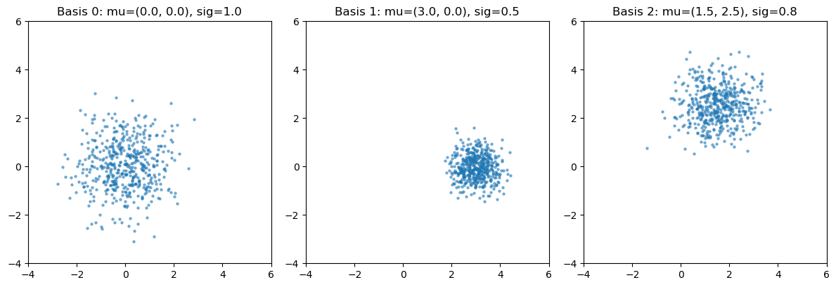
Three 2D Gaussians at different locations/scales as our “simulated” basis points.
# basis points in parameter space: (mu_x, mu_y, scale)
basis_params = [
    (0.0, 0.0, 1.0),   # centered, unit scale
    (3.0, 0.0, 0.5),   # shifted right, tight
    (1.5, 2.5, 0.8),   # shifted up-right
]

def sample_basis(idx, n):
    """Sample from basis distribution idx."""
    mu_x, mu_y, scale = basis_params[idx]
    mu = torch.tensor([mu_x, mu_y])
    return mu + scale * torch.randn(n, 2)

fig, axes = plt.subplots(1, 3, figsize=(12, 4))
for i, ax in enumerate(axes):
    data = sample_basis(i, 500).numpy()
    ax.scatter(data[:, 0], data[:, 1], s=5, alpha=0.5)
    ax.set_title(f"Basis {i}: mu=({basis_params[i][0]}, {basis_params[i][1]}), sig={basis_params[i][2]}")
    ax.set_xlim(-4, 6)
    ax.set_ylim(-4, 6)
    ax.set_aspect('equal')
plt.tight_layout()
plt.show()
2. Simple morphing model#
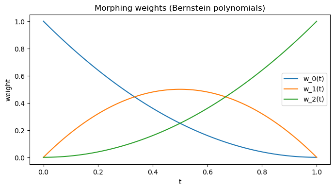
Parametrize by a single parameter \( t \in [0, 1]\) with quadratic Bernstein basis:
\(f_{0}(t) = (1-t)^{2}\)
\(f_{1}(t) = 2t(1-t)\)
\(f_{2}(t) = t^{2}\)
This gives Bézier-like interpolation link. Weights are always positive and sum to 1.
def morphing_weights(t):
    """Quadratic Bernstein basis"""
    t = torch.as_tensor(t, dtype=torch.float32)
    w0 = (1 - t) ** 2
    w1 = 2 * t * (1 - t)
    w2 = t ** 2
    return torch.stack([w0, w1, w2], dim=-1)

# weights vs t
ts = torch.linspace(0, 1, 100)
ws = morphing_weights(ts)
plt.figure(figsize=(8, 4))
for i in range(3):
    plt.plot(ts.numpy(), ws[:, i].numpy(), label=f"w_{i}(t)")
plt.xlabel("t")
plt.ylabel("weight")
plt.legend()
plt.title("Morphing weights (Bernstein polynomials)")
plt.show()
3. Train a flow for each basis distribution#
def train_flow(basis_idx, n_data=10000, n_steps=2000):
    """Train a flow on basis distribution."""
    data = sample_basis(basis_idx, n_data)
    field = nami.VelocityField(dim=2)
    optimizer = torch.optim.Adam(field.parameters(), lr=1e-3)
    for step in range(n_steps):
        x_source = torch.randn_like(data)
        loss = nami.fm_loss(field, data, x_source)
        optimizer.zero_grad()
        loss.backward()
        optimizer.step()

    base = nami.StandardNormal(event_shape=(2,))
    solver = nami.RK4(steps=32)
    fm = nami.FlowMatching(field, base, solver, event_ndim=1)
    print(f"Basis {basis_idx}: final loss = {loss.item():.4f}")
    return fm

# train all 3 flows
flows = [train_flow(i) for i in range(3)]
Basis 0: final loss = 1.5816
Basis 1: final loss = 0.7786
Basis 2: final loss = 1.2506
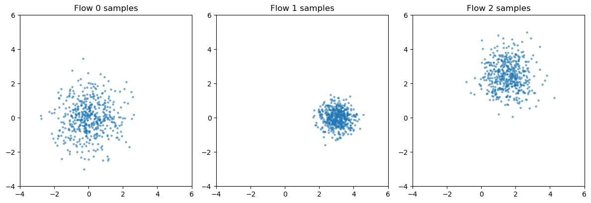
verify each flow learned its basis#
fig, axes = plt.subplots(1, 3, figsize=(12, 4))
for i, (ax, fm) in enumerate(zip(axes, flows)):
    samples = fm(None).sample((500,)).detach().numpy()
    ax.scatter(samples[:, 0], samples[:, 1], s=5, alpha=0.5)
    ax.set_title(f"Flow {i} samples")
    ax.set_xlim(-4, 6)
    ax.set_ylim(-4, 6)
    ax.set_aspect('equal')
plt.tight_layout()
plt.show()
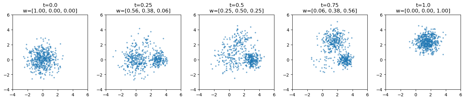
Morphed sampling at arbitrary t#
def morphed_sample(flows, t, n_samples):
    """Sample from morphed distribution at parameter t."""
    w = morphing_weights(t)

    # sample component indices according to weights
    k = torch.multinomial(w, n_samples, replacement=True)

    # collect samples from each component
    samples = []
    for i, fm in enumerate(flows):
        n_i = (k == i).sum().item()
        if n_i > 0:
            samples.append(fm(None).sample((n_i,)).detach())

    samples = torch.cat(samples)
    return samples[torch.randperm(len(samples))]


# show morphing at different t values
t_values = [0.0, 0.25, 0.5, 0.75, 1.0]
fig, axes = plt.subplots(1, 5, figsize=(15, 3))

for ax, t in zip(axes, t_values):
    samples = morphed_sample(flows, t, 500).numpy()
    ax.scatter(samples[:, 0], samples[:, 1], s=5, alpha=0.5)
    w = morphing_weights(t)
    ax.set_title(f"t={t}\nw=[{w[0]:.2f}, {w[1]:.2f}, {w[2]:.2f}]")
    ax.set_xlim(-4, 6)
    ax.set_ylim(-4, 6)
    ax.set_aspect('equal')

plt.tight_layout()
plt.show()
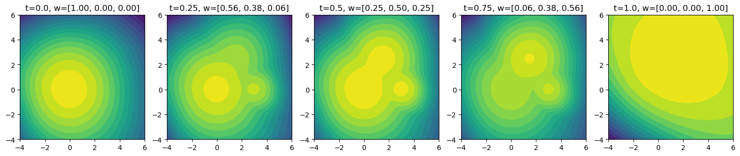
Morphed density evaluation#
def morphed_log_prob(x, flows, t):
    """Evaluate log p(x) at morphed parameter t."""
    w = morphing_weights(t)
    estimator = nami.HutchinsonDivergence()

    # get log probs from each component
    log_probs = torch.stack([
        fm(None).log_prob(x, estimator=estimator) for fm in flows
    ])  # (3, *batch)

    # Mixture --->  p = sum_k w_k p_k
    # so log p = logsumexp(log w_k + log p_k)
    log_w = w.log().view(-1, *([1] * (log_probs.ndim - 1)))
    return torch.logsumexp(log_w + log_probs, dim=0)


def plot_density(flows, t, ax, resolution=50):
    """Plot density contours at parameter t."""
    x = torch.linspace(-4, 6, resolution)
    y = torch.linspace(-4, 6, resolution)
    xx, yy = torch.meshgrid(x, y, indexing='xy')
    grid = torch.stack([xx.flatten(), yy.flatten()], dim=-1)
    with torch.no_grad():
        logp = morphed_log_prob(grid, flows, t)

    logp = logp.reshape(resolution, resolution).numpy()
    ax.contourf(xx.numpy(), yy.numpy(), logp, levels=20, cmap='viridis')
    w = morphing_weights(t)
    ax.set_title(f"t={t}, w=[{w[0]:.2f}, {w[1]:.2f}, {w[2]:.2f}]")
    ax.set_aspect('equal')


fig, axes = plt.subplots(1, 5, figsize=(15, 3))
for ax, t in zip(axes, t_values):
    plot_density(flows, t, ax)
plt.tight_layout()
plt.show()
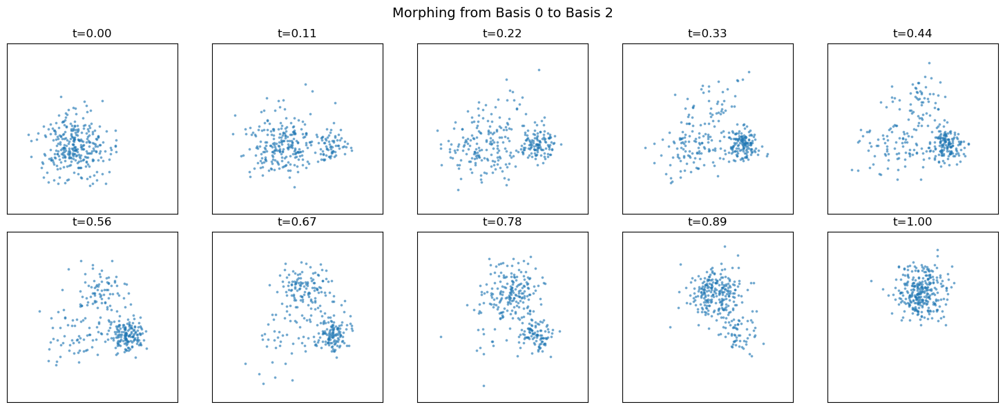
sweep through morphing parameter#
fig, axes = plt.subplots(2, 5, figsize=(15, 6))
t_sweep = torch.linspace(0, 1, 10)

for ax, t in zip(axes.flat, t_sweep):
    samples = morphed_sample(flows, t.item(), 300).numpy()
    ax.scatter(samples[:, 0], samples[:, 1], s=3, alpha=0.5)
    ax.set_title(f"t={t:.2f}")
    ax.set_xlim(-4, 6)
    ax.set_ylim(-4, 6)
    ax.set_aspect('equal')
    ax.set_xticks([])
    ax.set_yticks([])

plt.suptitle("Morphing from Basis 0 to Basis 2", fontsize=14)
plt.tight_layout()
plt.show()
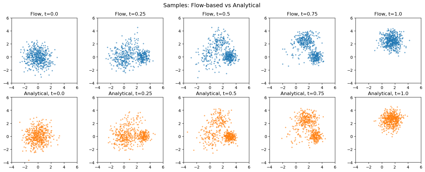
Compare to analytical Gaussian mixture#
Since our basis distributions are Gaussians, we can compute the exact morphed distribution analytically.
def analytical_sample(t, n_samples):
    """Sample from exact Gaussian mixture at parameter t."""
    w = morphing_weights(t)
    k = torch.multinomial(w, n_samples, replacement=True)
    samples = []
    for i, (mu_x, mu_y, scale) in enumerate(basis_params):
        n_i = (k == i).sum().item()
        if n_i > 0:
            mu = torch.tensor([mu_x, mu_y])
            samples.append(mu + scale * torch.randn(n_i, 2))

    samples = torch.cat(samples)
    return samples[torch.randperm(len(samples))]


def analytical_log_prob(x, t):
    """Exact log p(x) for Gaussian mixture at parameter t."""
    w = morphing_weights(t)

    log_probs = []
    for i, (mu_x, mu_y, scale) in enumerate(basis_params):
        mu = torch.tensor([mu_x, mu_y])
        # 2D isotropic Gaussian: log p = -0.5 * ||x-mu||^2/sigma^2 - log(2*pi*sigma^2)
        diff = x - mu
        log_p = -0.5 * (diff ** 2).sum(dim=-1) / (scale ** 2) - np.log(2 * np.pi * scale ** 2)
        log_probs.append(log_p)

    log_probs = torch.stack(log_probs)  # (3, *batch)
    log_w = w.log().view(-1, *([1] * (log_probs.ndim - 1)))
    return torch.logsumexp(log_w + log_probs, dim=0)
# flow vs analytical
fig, axes = plt.subplots(2, 5, figsize=(15, 6))

for col, t in enumerate(t_values):
    # flow samples (top row)
    ax_flow = axes[0, col]
    s_flow = morphed_sample(flows, t, 500).numpy()
    ax_flow.scatter(s_flow[:, 0], s_flow[:, 1], s=5, alpha=0.5, c='C0')
    ax_flow.set_title(f"Flow, t={t}")
    ax_flow.set_xlim(-4, 6)
    ax_flow.set_ylim(-4, 6)
    ax_flow.set_aspect('equal')

    # analytical samples (bottom row)
    ax_true = axes[1, col]
    s_true = analytical_sample(t, 500).numpy()
    ax_true.scatter(s_true[:, 0], s_true[:, 1], s=5, alpha=0.5, c='C1')
    ax_true.set_title(f"Analytical, t={t}")
    ax_true.set_xlim(-4, 6)
    ax_true.set_ylim(-4, 6)
    ax_true.set_aspect('equal')

plt.suptitle("Samples: Flow-based vs Analytical", fontsize=14)
plt.tight_layout()
plt.show()
# compare density contours
resolution = 60
x = torch.linspace(-4, 6, resolution)
y = torch.linspace(-4, 6, resolution)
xx, yy = torch.meshgrid(x, y, indexing='xy')
grid = torch.stack([xx.flatten(), yy.flatten()], dim=-1)

fig, axes = plt.subplots(2, 5, figsize=(15, 6))

for col, t in enumerate(t_values):
    ax_flow = axes[0, col]
    with torch.no_grad():
        logp_flow = morphed_log_prob(grid, flows, t)
    logp_flow = logp_flow.reshape(resolution, resolution).numpy()
    ax_flow.contourf(xx.numpy(), yy.numpy(), logp_flow, levels=20, cmap='viridis')
    ax_flow.set_title(f"Flow, t={t}")
    ax_flow.set_aspect('equal')

    ax_true = axes[1, col]
    logp_true = analytical_log_prob(grid, t).reshape(resolution, resolution).numpy()
    ax_true.contourf(xx.numpy(), yy.numpy(), logp_true, levels=20, cmap='viridis')
    ax_true.set_title(f"Analytical, t={t}")
    ax_true.set_aspect('equal')

plt.suptitle("Log-density: Flow-based vs Analytical", fontsize=14)
plt.tight_layout()
plt.show()
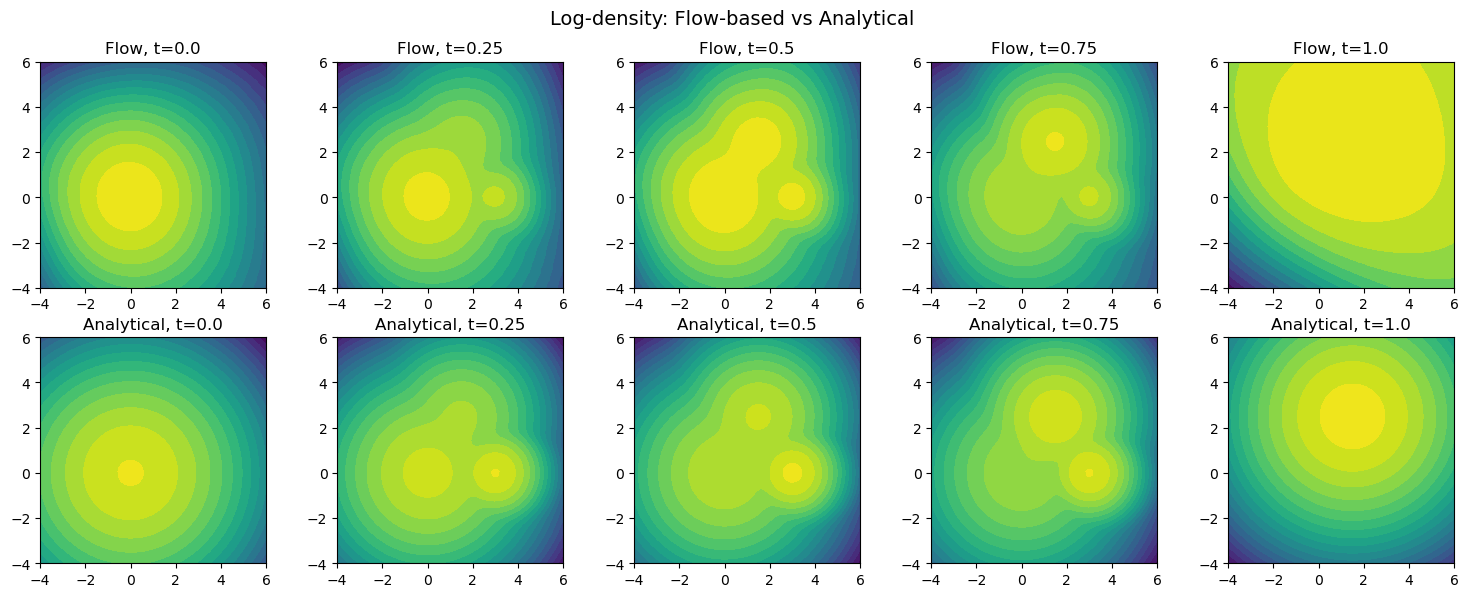
# MSE of log-prob on grid
print("MSE(log p_flow, log p_analytical) at each t:")
print("-" * 40)
for t in t_values:
    with torch.no_grad():
        logp_flow = morphed_log_prob(grid, flows, t)
    logp_true = analytical_log_prob(grid, t)

    # mask out very low density regions (where both are ~-inf)
    mask = logp_true > -20
    mse = ((logp_flow[mask] - logp_true[mask]) ** 2).mean().item()
    print(f"t={t:.2f}: MSE = {mse:.4f}")
MSE(log p_flow, log p_analytical) at each t:
----------------------------------------
t=0.00: MSE = 0.6654
t=0.25: MSE = 1.2286
t=0.50: MSE = 1.2685
t=0.75: MSE = 1.2822
t=1.00: MSE = 29.3668
so bad at boundary, weight loss for late times?
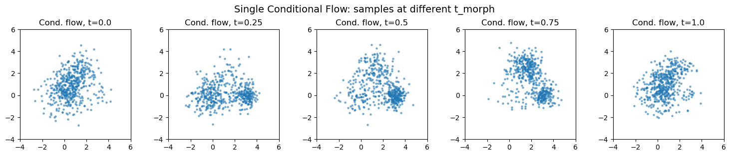
Single conditional flow#
Instead of 3 separate flows + mixture, train one flow conditioned on t. The network learns the morphing implicitly.
# use positional encoding for t_morph to make it more informative
class ConditionalVelocityField(nn.Module):
    def __init__(self, dim=2, cond_dim=1, hidden=128, n_freq=4):
        super().__init__()
        self.n_freq = n_freq
        # encode t_morph with sinusoidal features
        encoded_dim = 2 * n_freq  # sin/cos for each frequency

        self.net = nn.Sequential(
            nn.Linear(dim + 1 + encoded_dim, hidden),
            nn.SiLU(),
            nn.Linear(hidden, hidden),
            nn.SiLU(),
            nn.Linear(hidden, hidden),
            nn.SiLU(),
            nn.Linear(hidden, dim),
        )

    @property
    def event_ndim(self):
        return 1

    def encode_condition(self, c):
        """Encode scalar condition with positional encoding."""
        # c: (..., 1)
        c = c.squeeze(-1)  # (...,)
        freqs = torch.arange(1, self.n_freq + 1, device=c.device, dtype=c.dtype)
        angles = c.unsqueeze(-1) * freqs * 2 * torch.pi  # (..., n_freq)
        encoded = torch.cat([torch.sin(angles), torch.cos(angles)], dim=-1)  # (..., 2*n_freq)
        return encoded

    def forward(self, x, t, c):
        lead_shape = x.shape[:-1]

        if t.dim() == 0:
            t_exp = t.expand(*lead_shape).unsqueeze(-1)
        else:
            t_exp = t.unsqueeze(-1).expand(*lead_shape, 1)

        c_encoded = self.encode_condition(c)  # (..., 2*n_freq)

        inp = torch.cat([x, t_exp, c_encoded], dim=-1)
        return self.net(inp)
# ample (x, t_morph) pairs from the morphed distribution
cond_field = ConditionalVelocityField(
                dim=2,
                cond_dim=1,
                hidden=128,
                n_freq=8,
                )

optimizer = torch.optim.Adam(cond_field.parameters(), lr=1e-3)

n_steps = 10000
batch_size = 512

for step in range(n_steps):
    t_morph = torch.rand(batch_size)

    # for each t_morph, sample x from the corresponding mixture
    # (sample component k with prob w_k, then sample from that Gaussian)
    w = morphing_weights(t_morph)  # (batch, 3)
    k = torch.multinomial(w, 1).squeeze(-1)  # (batch,)

    # sample from selected basis Gaussians
    x_target = torch.zeros(batch_size, 2)
    for i, (mu_x, mu_y, scale) in enumerate(basis_params):
        mask = k == i
        n_i = mask.sum().item()
        if n_i > 0:
            mu = torch.tensor([mu_x, mu_y])
            x_target[mask] = mu + scale * torch.randn(n_i, 2)

    # standard flow matching training with condition
    x_source = torch.randn_like(x_target)
    c = t_morph.unsqueeze(-1)  # (batch, 1)

    loss = nami.fm_loss(cond_field, x_target, x_source, c=c)
    optimizer.zero_grad()
    loss.backward()
    optimizer.step()

    if step % 1000 == 0:
        print(f"Step {step}: loss = {loss.item():.4f}")

print(f"Final loss: {loss.item():.4f}")
Step 0: loss = 4.7810
Step 1000: loss = 2.0712
Step 2000: loss = 1.9316
Step 3000: loss = 1.7776
Step 4000: loss = 1.8576
Step 5000: loss = 1.7874
Step 6000: loss = 1.9675
Step 7000: loss = 1.8974
Step 8000: loss = 1.9011
Step 9000: loss = 1.9868
Final loss: 1.9760
# BoundField: stores conditioning, creates tensor matching x's leading dims
class BoundField(nn.Module):
    def __init__(self, field, c):
        super().__init__()
        self._field = field
        self._c_value = float(c.view(-1)[0].item())

    @property
    def event_ndim(self):
        return self._field.event_ndim

    def forward(self, x, t, c=None):
        # Create c matching x's leading dims: x=(sample, batch, event) -> c=(sample, batch, 1)
        lead_shape = x.shape[:-1]
        c_new = torch.full((*lead_shape, 1), self._c_value, device=x.device, dtype=x.dtype)
        return self._field(x, t, c_new)
# create a LazyField wrapper that binds conditioning
class ConditionedLazyField(nami.LazyField):
    def __init__(self, field):
        super().__init__()
        self._field = field

    @property
    def event_ndim(self):
        return self._field.event_ndim

    def forward(self, c):
        """Return a bound field that has c baked in."""
        return BoundField(self._field, c)

# create conditional FlowMatching
base = nami.StandardNormal(event_shape=(2,))
solver = nami.RK4(steps=32)

cond_fm = nami.FlowMatching(
    ConditionedLazyField(cond_field),
    base,
    solver,
    event_ndim=1
)
# Sample from conditional flow at different t_morph values
fig, axes = plt.subplots(1, 5, figsize=(15, 3))

for ax, t in zip(axes, t_values):
    # Condition tensor: shape (1, 1) for single t_morph value
    c = torch.tensor([[t]])

    # Sample via conditioned flow - this gives (500, 1, 2)
    samples = cond_fm(c).sample((500,)).detach().numpy()

    # Squeeze the batch dimension: (500, 1, 2) -> (500, 2)
    samples = samples.squeeze(1)

    ax.scatter(samples[:, 0], samples[:, 1], s=5, alpha=0.5)
    ax.set_title(f"Cond. flow, t={t}")
    ax.set_xlim(-4, 6)
    ax.set_ylim(-4, 6)
    ax.set_aspect('equal')

plt.suptitle("Single Conditional Flow: samples at different t_morph", fontsize=14)
plt.tight_layout()
plt.show()
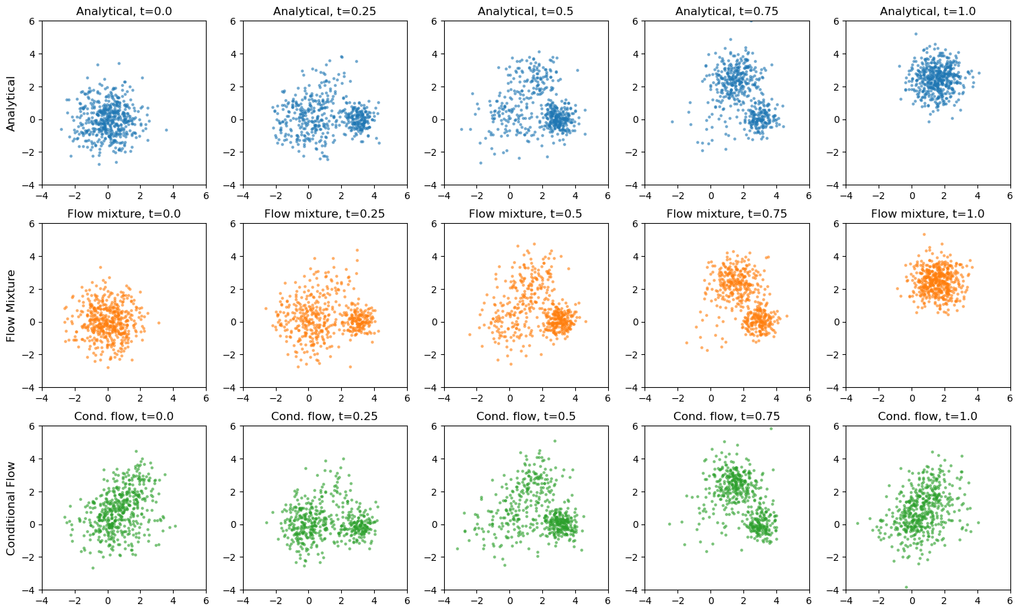
# compare all 3 approaches: Analytical vs Flow Mixture vs Conditional Flow
fig, axes = plt.subplots(3, 5, figsize=(15, 9))

for col, t in enumerate(t_values):
    # Row 0: Ana
    ax = axes[0, col]
    s = analytical_sample(t, 500).numpy()
    ax.scatter(s[:, 0], s[:, 1], s=5, alpha=0.5, c='C0')
    ax.set_title(f"Analytical, t={t}")
    ax.set_xlim(-4, 6)
    ax.set_ylim(-4, 6)
    ax.set_aspect('equal')

    # Row 1: Flow mixture
    ax = axes[1, col]
    s = morphed_sample(flows, t, 500).numpy()
    ax.scatter(s[:, 0], s[:, 1], s=5, alpha=0.5, c='C1')
    ax.set_title(f"Flow mixture, t={t}")
    ax.set_xlim(-4, 6)
    ax.set_ylim(-4, 6)
    ax.set_aspect('equal')

    # Row 2: Conditional flow
    ax = axes[2, col]
    c = torch.tensor([[t]])
    s = cond_fm(c).sample((500,)).detach().numpy()
    s = s.squeeze(1)
    ax.scatter(s[:, 0], s[:, 1], s=5, alpha=0.5, c='C2')
    ax.set_title(f"Cond. flow, t={t}")
    ax.set_xlim(-4, 6)
    ax.set_ylim(-4, 6)
    ax.set_aspect('equal')

axes[0, 0].set_ylabel("Analytical", fontsize=12)
axes[1, 0].set_ylabel("Flow Mixture", fontsize=12)
axes[2, 0].set_ylabel("Conditional Flow", fontsize=12)
plt.tight_layout()
plt.show()
# auantitative: MSE comparison for conditional flow
def cond_flow_log_prob(x, t_morph):
    """Log prob from conditional flow at t_morph."""
    c = torch.full((x.shape[0], 1), t_morph)
    estimator = nami.HutchinsonDivergence()
    return cond_fm(c[:1]).log_prob(x, estimator=estimator)

print("MSE comparison: Flow Mixture vs Conditional Flow")
print(f"{'t':<6} {'Mixture MSE':<15} {'Cond. Flow MSE':<15}")
print("-" * 50)

for t in t_values:
    logp_true = analytical_log_prob(grid, t)
    mask = logp_true > -20

    with torch.no_grad():
        logp_mix = morphed_log_prob(grid, flows, t)
    mse_mix = ((logp_mix[mask] - logp_true[mask]) ** 2).mean().item()

    with torch.no_grad():
        logp_cond = cond_flow_log_prob(grid, t)
    mse_cond = ((logp_cond[mask] - logp_true[mask]) ** 2).mean().item()

    print(f"{t:<6.2f} {mse_mix:<15.4f} {mse_cond:<15.4f}")
MSE comparison: Flow Mixture vs Conditional Flow
t      Mixture MSE     Cond. Flow MSE
--------------------------------------------------
0.00   0.6654          16.0255
0.25   1.2288          3.4486
0.50   1.2680          3.7996
0.75   1.2811          3.2058
1.00   29.3404         33.5013
flow Mixture vs Conditional Flow#
The conditional flow learns the entire family of distributions p(x|t) in one model, enabling Gradient-based inference (\(\partial \log p / \partial t\)), smooth interpolation between any parameter values, but condiioning needs to be right.
# check variance of flow 2's log_prob
logps = []
for _ in range(10):
    with torch.no_grad():
        logps.append(flows[2](None).log_prob(grid, estimator=nami.HutchinsonDivergence()))
logps = torch.stack(logps)
print(f"Std of log_prob estimates: {logps.std(dim=0).mean():.4f}")
Std of log_prob estimates: 0.0401
# direct comparison for basis 2 only
logp_flow2 = flows[2](None).log_prob(grid, estimator=nami.HutchinsonDivergence())
mu = torch.tensor([1.5, 2.5])
scale = 0.8
logp_true2 = -0.5 * ((grid - mu) ** 2).sum(-1) / scale**2 - np.log(2 * np.pi * scale**2)

mask = logp_true2 > -20
print(f"Flow 2 MSE: {((logp_flow2[mask] - logp_true2[mask])**2).mean():.4f}")
Flow 2 MSE: 29.3466